C&A LAB

Notice

This post is a summary of a presentation entitled 'What is Dataset Distillation' at C&A Lab 2023-Summer Deep Learning Seminar. The corresponding slide is available at Here.

As can be inferred from the title of the presentation, this post contains an introduction to Dataset Distillation. And The following papers will be covered in order.

For the sake of length and readability, I will only post some papers at a time. In this post, the underlined [TJA+18] will be introduced.

- [TJA+18] Dataset Distillation, (arXiv’18)

- [ZMB21] Dataset Condensation with Gradient Matching, (ICLR’21)

- [ZB21] Dataset Condensation with Differentiable Siamese Augmentation, (ICML’ 21)

- [ZB23] Dataset Condensation with Distribution Matching, (WACV’ 23)

- [CWT+23] Dataset Distillation by Matching Training Trajectories, (CVPRW’ 23)

Intro

As generally known, the development of deep learning has made it possible to pursue high performance and good convenience in many application cases. In addition, there have been many studies on performance improvement and good application, and generally high performance can be achieved by training heavier models with a lot of training data. However, it is clear that the exponential increase in model complexity is not only a good thing. Slower input passing through the model means that the model trains or evaluate slower, and the increased size of the model also means that it is more cumbersome to store.

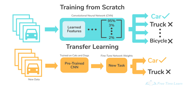
Accordingly, researchers began to pay attention to lightweight models. However, it is known that using the existing general model training method as it is to train a lightweight model results in poor performance. As a solution to this, a technique for model distillation (knowledge distillation) has been introduced, and learning is generally conducted in such a way that the pre-trained teacher model's knowledge is transferred to the student model. This idea is now a kind of research field and is actively being researched.

However, [TJA+18] proceeds with related but orthogonal tasks. The main idea is to synthesize a small number of data points that do not need to come from the correct data distribution, but will, when given to the learning algorithm as training data, approximate the model trained on the original paper. There is a toy figure for supporting to understand.

For example, the MNIST dataset, which includes 10 classes and a total of 60,000 training images, is compressed into one synthetic data per class to train the model with only 10 images.

In the case of a model trained using the entire dataset, it showed 99% accuracy, but it is said that 94% accuracy was obtained when the same model was trained with only 10 images that went through dataset distillation.

Approach

For explanation, there is some notation as follows:

$\mathbf{x}=\{x_i\}_{i=1}^{N}$ : train dataset

$\theta$ : neural network parameters

$l(x_i,\theta)$ : loss function

Also, basic task is image classification as follows:

- Optimizing distilled data

Using these learned synthetic data can greatly boost the performance on the real test set. Given an initial $\theta_0$, we obtain these synthetic data $\tilde{\mathbf{x}}$ and learning rate $\tilde{\eta}$ by minimizing the objective below $L$:

- Distillation for random initialization

Distilled data for a given initial value does not generalize to another initial value. The data distilled by encoding information about the training dataset x and a particular network initialization often looks like random noise. To solve this problem, a small number of distilled data was synthesized in a way that the network could operate even according to a random initial value according to a specific distribution.

- Distillation with with different initializations

Random initialization : A distribution of random initial weights. For example, HE Initialization and Xavier Initialization in neural networks.
Fixed initialization : A specific fixed network initialization method from above.
Random pre-trained weights : The distribution of pre-trained models on different tasks or datasets. For example, there is AlexNet pre-trained on ImageNet.
Fixed pre-trained weights : A network that has been pre-trained on a different task or dataset and is specifically fixed.

- Main algorithm

The main algorithm is as follows:

Experiment

- Baselines

Random real images: Take the same number of random samples per category from real images.
Optimized real images: After constructing several random sets based on the criteria set above, the set with the top 20% performance is selected.
k-means: Apply k-means clustering for each category, and use the center of the cluster as a training image.
Average real images: Calculates the average image for each category, which is reused in other gradient descent steps.

- Fixed Initialization: When experimenting with Dataset Distillation compressed with only one image per class with only 1 epoch

- Random Initialization : Test results of Dataset Distillation dataset obtained through 3 epoch

- Comparison between Dataset distillation dataset trained for ten GD steps and three epochs and various baselines

- Other Experiments

Several experiments using the method are provided in the paper. Among the things confirmed in various experiments, experiments on hyperparameter settings (steps, epochs) required for dataset distillation, accuracy and convergence trend as the number of images per class increased, and tuning to pre-learned parameters with different data sets for the same task There are experiments such as the fact that adoption is possible with dataset distillation data, and that it is possible to create data that hinders learning by using the intuition of creating data that is conducive to learning. For more details, please check the original paper(Link).

Conclusion

This paper has the greatest contribution by presenting the concept of dataset distillation for the first time. However, the method presented in this study is expected to take a long time to implement and require large amounts of memory in using images as learning parameters. In addition, it can be considered that the difference in performance from the original data is obvious, and an effort was made to solve the dependence of the initial setting of the parameters, but additional research is needed.

Introduction

NOTE. This post is a summary of a presentation entitled "Understanding Adversarial Examples" at "C&A Lab 2023-Summer Deep Learning Seminar". The corresponding slide is available at HERE.

ALSO NOTE. This is the third post for "Understanding Adversarial Examples." If you have not read my previous posts, then it would be beneficial to read them for the sake of better understanding! The links are available below.

- (1st Post) Adversarial Robustness as a Prior for Learned Representations
- (2nd Post) Do Adversarially Robust ImageNet Models Transfer Better?

So far, we have continued our journey toward understanding adversarial examples by reviewing two previous papers that elaborated on identifying the properties of adversarially robust classifiers. However, we did not yet address an important and ultimate question: So, why do adversarial examples exist? Are they an inevitable, natural consequence of learning itself or just an imperfection of the current machine learning algorithm?

In this post, I introduce a paper that gives some insights into how to answer the aforementioned question through so-called shortcut learning.

- [EIS+19] Adversarial Robustness as a Prior for Learned Representations (arXiv'19)

- [SIE+20] Do Adversarially Robust ImageNet Models Transfer Better? (NIPS'20)

- [GJM+20] Short-cut Learning (Nature MI'20)

- [HZB+21] Natural Adversarial Examples (CVPR'21)

What is Short-cut Learning?

In general, short-cut learning refers to the tendency to learn "spurious cues" during training. Historically, there have been several examples of short-cut learning, such as the clever Hans effect.

In the theory of education, short-cut learning is also related to the notion called surface learning. Consider a history exam that consists of problems asking the precise year of each historical event, e.g., when America became free from England? In order to get a good grade on this exam, it would be beneficial to simply memorize all the numbers in the chronology, rather than understand the causality, implication, and importance of each event. Now consider two students, Alice and Bob, studied by these two strategies, respectively. Alice would get a better grade than Bob in this exam, but is it fair to conclude that Alice is better than Bob in History?

The aforementioned examples correspond to biological neural networks (Yes, our brain!). Then, how about neural networks? We can observe several examples that could "fool" the target classifier. We already called them "Adversarial Examples". Moreover, several studies have reported that even well-chosen natural images can fool the classifier (Spoiler Alert: I will review a paper that provides an in-depth analysis of this phenomenon in the next post!). In addition, other works have demonstrated that the classifier trained by ImageNet is prone to becomeing biased towards the texture of the given image, or that the background of the given object may play a significant role in the decision of the neural network.

A simple toy example of the occurrence of short-cut learning is provided. Let us consider two datasets, each of which consists of stars and moons in specific positions, respectively. Our goal is to train a neural network from two datasets in order to determine whether the given image contains a star or moon. However, the configuration of the dataset would be different from our original intention: As we can figure out in the picture below, the star only appears in the left lower and right upper corners of the image, whereas the moon does in the right lower and left upper corners. If the neural network catches these "positional" characteristics rather than the shapes of each object, then the neural network would give an unintended solution in the red box.

A Journey for finding a Good Solution

Now, what is a good solution that the neural network should learn? For the given task, there are infinitely many solutions that might work well. Nevertheless, it cannot be ensured that all the solutions could be generalized well; maybe there are a lot of shortcuts in these solutions. This paper formalizes each solution as a "decision rule", a strategy to solve the given task that the neural network would learn. According to their study, such a decision rule could be classified into four categories, each of which is stated as follows:

- Level 1. Uninformative Features: They cannot solve even the given task.
- Level 2. Overfitting Features: They solve a given task, but it becomes useless when we consider other tasks i.i.d. (identically, independently distributed) from the initial task. (Train Dataset vs. Test Dataset configured by dividing a single dataset.)

- Level 3. Shortcut Feautres: They solve a given task, along with good results from i.i.d. test dataset. However, they cannot solve the tasks from o.o.d. (out-of-distribution). (ImageNet vs. CIFAR10)

- Level 4. Intended Features: They are desired solutions that would be generalized well even for tasks from o.o.d..

For a better understanding, an overview figure is as follows:

Why Short-cut Learning Occurs in NNs?

Then, where do the shortcuts come from? This paper suggested two types of shortcut learning in terms of the training datasets and decision rules.

From the point of view of the dataset, they considered an effect of the "soundness" of the dataset using the term "shortcut opportunities". The dataset itself contains the direction of the learning. However, as we saw in the examples of shortcut learning in biological neural networks, shortcut learning can occur as surface learning in education when the train set (questions in the exam) is not made properly. It is not an exception in the case of image classification tasks; In general, the image of sheep would be presented with a background of grasses. Of course, this might be helpful in the model's decision, but at the same time, this would enable the model to learn a spurious cue from the grass. Even worse, these shortcut opportunities can arise in other forms, such as the context, e.g., it is natural to wear socks on the foot rather than on the head. In fact, there is a study [1] on the effect of backgrounds onthe image classification task. The following image shows that the BG (Background) of the given image also plays an important role as the FG (Foreground).

On the other hand, from perspective of decision rule, they give an example of how the model can learn somewhat biased features from the given dataset. Although this phenomenon would be architecture-dependent, a recent notable study [2] demonstrated that the CNN-based classifiers trained with the ImageNet dataset are prone to being biased by texture information. The following figure indicates that if the texture (elephant) and the context (cat) collide in the given image, then the decision of the classifier is relatively more dependent on the texture.

So what? Why does shortcut learning occur? There are several candidates to demystify the reason for shortcut learning in neural networks, but unfortunately, clearly understanding each of them is an open problem. Nevertheless, we can investigate the effect of each fundamental component for training neural networks part by part: The architecture of the neural network, the configuration of the training data, the choice of the loss function, and the choice of the optimizer.

To explain the shortcut opportunities, there is a well-known principle in various research realms, called "the principle of less effort." In many tasks, including learning, web surfing, or searching the library, everyone (even machines!) is trying to minimize their effort to get a desirable result. From this point of view, harnessing shortcut opportunities can be understood as a consequence of the principle of less effort that the neural network adopted during training.

For decision rules, other fundamental components could be taken into account: in terms of architecture, inductive bias could be considered a reason for shortcut learning. Compared to CNNs, vision transformers have a less inductive bias in terms of collecting local information about the given image. Extensive analyses on the effect of the architecture of neural networks are also a classical but good research topic, but the computational cost of training each model would be expensive. Also, the choice of loss function, including regularization technique, or optimizer, including the choice of learning rate, can be factors in the occurrence of shortcut learning. However, current works are not yet mature enough to fully analyze the effects; only simpler models (shallow-layered neural networks) have been studied, so analyzing them in deeper, more complex neural networks is an open problem.

Comment & Discussion

This paper gives a quick overview of the shortcut learning that appears in neural networks. Shortcut learning itself seems like a quite natural consequence of learning, but it is an important obstacle to overcome for the sake of trustworthy AI. According to their paper, they used the expression "connecting the dots" to understand several peculiar phenomena we have observed during understanding the inner-workings of neural network. Although they look independent each other at a glance, in terms of shortcut learning, some problems may have an implicit "bridge" called shortcut learning.

In my opinion, a good starting point to figure out such bridges is to understand the relation between the adversarial examples and the membership inference attack, which is an attack to determine whether the given data is used to train the target neural network. Remark that although these two types of attacks have been developed independently, some recent studies have pointed out that there is a certain relationship between them, so they mentioned that understanding them under the same framework would be an interesting but rather challenging future work.

To the best of my knowledge, a typical approach for membership inference attacks is to utilize the target model's sensitivity to the given input; intuitively, the model may give a more distinctive answer for the data when seen during training, compared to one never seen before. In the language of shortcut learning, this strategy can be understood as an attempt to find the gap between the train dataset and the i.i.d. or o.o.d. test set with respect to the model's decision rule.

Whereas adversarial examples are trying to generate data that makes the target model not behave as expected. This can be understood as a process to find an o.o.d. that the decision rule of the target model cannot cover. From this point of view, one may suspect that they are essentially the same type of attacks, except for the attacker's goal.

I think that there are other problems that could be connected to the bridge of shortcut learning. Honestly, I have no idea at the moment when I write this post, It would be an intriguing future work :)

References

[1] Xiao, K., Engstrom, L., Ilyas, A., & Madry, A. (2020). Noise or signal: The role of image backgrounds in object recognition. arXiv preprint arXiv:2006.09994.
[2] Geirhos, R., Rubisch, P., Michaelis, C., Bethge, M., Wichmann, F. A., & Brendel, W. (2018). ImageNet-trained CNNs are biased towards texture; increasing shape bias improves accuracy and robustness. arXiv preprint arXiv:1811.12231.

C&A Lab.

Deep Learning Seminar, 2023 Summer

Title: Iris Recognition(slide)

Date: 2023-08-02

Introduction.

The iris is a structure in the eyes, that is located between the pupil and the sclera(or the cornea). It is a well-known fact that the iris can be used to identify individuals, since the iris is made by combining fibrous tissue so that there are many different iris patterns.

The iris recognition is one of most popular biometric authentication system. According to data released by the Korea Financial Telecommunications and Clearings Institute(KFTC), the iris recognition is one of biometric recognition system with lowest false rejection rate and false acceptance rate(source).

Despite the high accuracy of iris recognition, very few consumers use iris recognition according to the result analyzed by Samsung Electronics(source). Even the German hacker group Chaos Computer Club (CCC) announced that it had succeeded in hacking iris recognition(source).

From these domestic and international circumstances, there are several limitations for iris recognition in terms of user convenience and security. Therefore, we investigate the research trends of the iris recognition in this post and its attack/protection techniques in the next post. In this post, we report a classical iris recognition: IrisCode(TPAMI'93), and a deep learning-based iris recognition: UniNet(ICCV'17).

1. Classical Iris Recognition(IrisCode)

The IrisCode is proposed by John Daugman in 1993, and its variants are still used a lot these days. In short, the IrisCode represents an iris for 2048-bit codes, as shown in the figure visualized above.

Informally, there are two steps, segmentation and encoding; the segmentation is to search for the iris boundary and detect the iris region, and the encoding is a process of extracting features from the region detected in the segmentation and encoding them into 2048-bit codes. A detailed explanation of each step is as follows.

1.1 Segmentation

The goal of segmentation is to find an inner and outer boundaries of an iris. The boundaries are found by the Daugman's integro-differential operator:

$$\max_{(r, {x}_{0}, {y}_{0})} \lvert {G}_{\sigma}(r) * \frac{\partial}{\partial r} \oint_{r,{x}_{0},{y}_{0}} \frac{I(x,y)}{2\pi r} ds \rvert$$

where G is a smoothing function, * is a convolution operation, I(x, y) is a raw image over a pixel domain and $(x_{0}, y_{0})$ is an center estimated for each radius r.

Gaussian of scale is used as a smoothing function, which plays a role in estimating the outer boundary and blurring the sclera. For each estimation, the contour integration of I(x, y) is conducted to search for the inner boundary. The values $(r, x_{0}, y_{0})$ are set to maximum in the blurred partial derivative of the contour integration.

1.2 Encoding

For encoding the iris region, the author applies a 2D Gabor filter, which is a methodology of extraction features from the image. Given feature points in the image, the 2D Gabor filter extracts the information along the direction from the location of the feature points and represents the result as a complex value. While the original 2D Gabor filter is defined over the pixel coordinates, the author projects the pixels of the image to polar coordinate system with $r \in [0,1]$ and $\theta \in [0, 2\pi]$, because the iris region is a circular shape. The equation of 2D Gabor filter in the IrisCode is as follows:

$$G(r, \theta)=e^{-\{ {(r-{r}_{0})}^{2}/{\alpha}^{2}+(\theta-{\theta}_{0})^{2}/{\beta}^{2}\}}e^{-i\omega(\theta-{\theta}_{0})}$$

where $(r_{0}, \theta_{0})$ is an feature point, $\alpha, \beta$ are parameters for frequency, and $\omega$ is a parameter for a direction.

The 2D Gabor filter is applied for each local region $I(\rho, \phi)$, and each sign of both the real and imaginary parts of the result becomes each bit in an IrisCode:

$${h}_{\{\mathrm{Re, Im}\}}=\mathrm{sgn}_{\{\mathrm{Re, Im}\}} \Bigg[\int_{\rho}\int_{\phi}e^{-\{{(\rho-{r}_{0})}^{2}/{\alpha}^{2}+(\phi-{\theta}_{0})^{2}/{\beta}^{2}\}}e^{-i\omega(\phi-{\theta}_{0})}\Bigg] $$

They argue that it takes 100 milliseconds to generate an IrisCode, that is 2048-bit codes for an iris.

1.3 Performance

IrisCode uses the normalized hamming distance as a matching metric. The authors of the paper present the performance of IrisCode under various HD criterions, which are decision thresholds of hamming distance for verification:

They report on the best result obtained when HD criterion is 0.32; the rate of false accept is 1/151000 and the rate of false reject is 1/128000. However, the above results seem to require additional analysis because the database or source code they used has not been disclosed.

2. DL-based Iris Recognition(UniNet)

2.1 Overview

Deep Learning(DL)-based image recognition is recently applied for the iris recognition system. UniNet is one of them, that point out the limitation of IrisCodes; they rely heavily on parameter selections when applied for different databases. On the other hand, the authors of UniNet argue that the typical deep learning architecture may not be optimal for iris, since they are not designed for the characteristics of the iris; there are no structural properties in the irises, unlike faces.

Therefore, they propose the UniNet by training the Extended Triplet Loss(ETL) to address the characteristics of iris pattern, with experiments on various databases. UniNet extracts features from the normalized images, and they uses the existing method for normalizing raw images. Examples for the dataset they used and the normalized image are shown in the figure below:

2.2 Architecture

UniNet is consist of two subnetworks, FeatNet and MaskNet. The former is a feature extraction from the normalized iris image, and the latter is a detection the iris region. Both are based on the structure of Fully Convolutional Neural Network(FCNN), which is a network without the fully-connected layer to preserve the local information in the image.

At first, the MaskNet is pre-trained by a pixelwise softmax loss, to conduct the binary classification to an iris region or non-iris region. The non-iris region indicates that the region covered by the eyelid in the normalized iris image. After training the MaskNet, the FeatNet is trained by their proposed loss function, Extended Triplet Loss(ETL) modifying the triplet loss.

2.3 Extended Triplet Loss(ETL)

The basic idea of ETL is same as the triplet loss, to make distances between feature maps from positive samples close and distances between feature maps from negative samples far. Therefore, ETL takes three samples as same as the triplet loss: anchor, positive and negative samples.

The following equations are the triplet loss and ETL.

$$L=\frac{1}{N}\sum_{i=1}^{N}{\Bigg[{||{f}_{i}^{A}-{f}_{i}^{P}||}^{2}-{||{f}_{i}^{A}-{f}_{i}^{N}||}^{2}+\alpha \Bigg]}_{+}$$

$$ETL=\frac{1}{N}\sum_{i=1}^{N}{\Bigg[{D({f}_{i}^{A}-{f}_{i}^{P})}^{2}-{D({f}_{i}^{A}-{f}_{i}^{N})}^{2}+\alpha \Bigg]}_{+}$$

where $N$ is the number of whole samples, $(f^{A}, f^{P}, f^{N})$ are feature maps corresponding to an anchor, positive and negative sample, $||\cdot||$ is the L2 norm and $\alpha$ is a margin. They modify the distance function, the L2 norm, to Minimum Shifted and Masked Distance function $D$:

$$D({f}^{1}, {f}^{2})=\min_{-B\leq b \leq B}\{FD({f}_{b}^{1},{f}^{2})\}$$

$$FD({f}^{1}, {f}^{2})=\frac{1}{|M|}\sum_{(x,y)\in M}{({f}_{x,y}^{1}-{f}_{x,y}^{2})}^{2}$$

where $m^{1}, m^{2}$ are the binary masks from the MaskNet corresponding feature maps $f^{1}, f^{2}$.

$D$ is defined by the fractional distance $FD$, which is masking the non-iris region along the output of MaskNet. In the above equation of $FD$, $M$ indicates that the only iris region.

In the equation of $D$, $b$ is the number of pixels shifted horizontally and $f_{b}$ is the feature map shifted by $b$ pixels from $f$. This is because that the horizontal translation usually exist between various normalized images from a same iris:

Finally, $D$ is defined with the minimum $b$ in the each positive and negative samples. Therefore, the function $D$ plays a role of shifting the minimum pixels and masking the non-iris region.

2.4 Encoding

They encodes the real-valued feature maps output from UniNet into binary features, since the binary features are more popular in the research on previous iris recognitions.

At first, the mean value is calculated in the non-iris region along the output from MaskNet. After that, each value of output from the FeatNet is binarized to 1 if the value is larger that the mean(iris region) or 0 otherwise(non-iris region). They adds a margin $t$ between the iris and non-iris region, and this marginal area is regarded as the non-iris region.

In the matching the outputs from FeatNet and MaskNet, they use the fractional Hamming distance, which is the normalized hamming distance. The bits of the output from FeatNet with minimum distance is selected the bits of the final feature, including the only iris region.

2.5 Comparison

2.5.1 Comparison with IrisCodes

They compare their performance with the existing IrisCodes: OSIRIS, log-Gabor, and Ordinal. The OSIRIS is an implementation for Daugman's IrisCode, and the log-Gabor and Ordinal are variants of IrisCode with modified Gabor filters. They outperform the these IrisCodes on the various databases.

In their method, CrossDB indicates that a training database is different from a test database, and WithinDB indicates that they fine-tuned the pre-trained UniNet with a part of the test database. WithinDB shows the slightly better performance than CrossDB.

2.5.2 Comparison with DeepIrisNet

They also presents the experiments of various backbones: FCN or CNN, and various loss functions: ETL, triplet loss, or softmax. They argue that FCN+ETL(Ours) shows the best performance among the combinations of a backbone and loss function as the figure below:

In the above figure, DeepIrisNet is one of DL-based iris recognition, that uses CNN and softmax as a loss function. They presents the comparison with DeepIrisNet in terms of parameters, storage, and time, since DeepIrisNet is specifically proposed for iris recognition:

3. Conclusion

While the DL-based face recognition is widely used in practice, DL-based iris recognition is challenging now. We expect that the capability of DL-based method can be applied for improving the limitations of the previous iris recognitions. It would be great to achieve maintaining security and accuracy while improving efficiency.

One of main direction is a research on the protection method from the various attack on iris recognition. The attack and protection method for iris recognition will be continued in the next post. :)

Reference.

[1] Daugman, J. G. (1993). High confidence visual recognition of persons by a test of statistical independence. IEEE transactions on pattern analysis and machine intelligence, 15(11), 1148-1161.

[2] Zhao, Z., & Kumar, A. (2017). Towards more accurate iris recognition using deeply learned spatially corresponding features. In Proceedings of the IEEE international conference on computer vision (pp. 3809-3818).

Introduction

NOTE. This post is a summary of a presentation entitled "Understanding Adversarial Examples" at "C&A Lab 2023-Summer Deep Learning Seminar". The corresponding slide is available at HERE.

ALSO NOTE. This is the second post for "Understanding Adversarial Examples." If you did not read my first post, then it would be beneficial to read that for the sake of better understanding!

When training a neural network with deep learning, the amount of available data plays an important role in the performance of the resultant network. Of course, for some tasks, such as image classification on web-crawled data or recognizing the facial images of celebrities, collecting sufficient, large data for training is not that difficult. However, on the other hand, there are still many tasks where collecting a large-scale dataset is almost impossible, such as medical data or biometrics data that requires special equipment for collecting the data, e.g., finger veins.

To address this problem, several solutions would be considered. For example, some studies elaborated on creating a synthetic dataset for exploiting recent sophisticated generative modeling techniques. But one traditional and simple approach is transfer learning. Transfer learning is an important branch of deep learning literature. By fine-tuning the pre-trained network for a task where a large number of data can be easily collected, i.e., image classification via the ImageNet dataset, the tuned network could obtain better accuracy with a smaller amount of data. The following simple figure briefly illustrates how transfer learning works:

At that moment, an important question follows: What should we do to improve transfer learning, and what is the main reason for its success? In this post, I will present the second paper that identifies the relationship between transfer learning and the adversarially robust model.

- [EIS+19] Adversarial Robustness as a Prior for Learned Representations (arXiv'19)

- [SIE+20] Do Adversarially Robust ImageNet Models Transfer Better? (NIPS'20)

- [GJM+20] Short-cut Learning (Nature MI'20)

- [HZB+21] Natural Adversarial Examples (CVPR'21)

Do Adversarially Robust ImageNet Models Transfer Better?

Conventional wisdom says that the main factor of enhancing the accuracy of transfer learning in the downstream task is the accuracy of the pre-trained model in the upstream task: A better pre-trained model would transfer its knowledge better. It would be correct if these two tasks were not that different, more precisely, if the distribution of each dataset was quite similar. However, this is not the case in many applications of transfer learning.

Then, for the sake of better transfer, what are the desirable properties that the pre-trained model would have? In terms of representation learning, it would be reasonable to consider whether the pre-trained model learned reasonable, robust representations from an upstream task.

As we saw in my first post, it is experimentally verified that the adversarially robust classification model has several advantages in terms of learned representation, including better representation inversion, direct visualization of representations, or feature interpolation. From this point of view, it seems natural to infer that robustness plays a significant role in the success of transfer learning.

This paper is the first study to elaborate on the aforementioned perspective. They conducted extensive analyses of various downstream tasks to demonstrate the effectiveness of adversarially robust models in transfer learning. Moreover, they provided several analyses and discussions, including the relation between the extent of robustness and the "granularity" of the dataset, and the correlation of the accuracy between the pre-trained model on the upstream task and the fine-tuned model on the downstream task when the notion of robustness is engaged. The following table is a quick summary of the contribution of this paper:

Experimental Setting

Transfer learning can be classified into two types with respect to the frozen parameters during fine-tuning: Fixed transfer learning and full transfer learning. The former freezes all parameters of the pre-trained model except those of the last layer, whereas the latter trains all parameters during fine-tuning.

In the sense of the robustly trained pre-trained model, it seems more natural to consider the fixed transfer learning setting than its counterpart, because it cannot be ensured that the adversarial robustness is preserved during full transfer learning. In addition, from the perspective of the robust feature model proposed by their previous study [IST+19], fixed transfer learning itself could be understood as a fine-tuning of the classifier without modifying the previously learned robust features.

However, they considered these two settings simultaneously because there was evidence that there is a positive correlation between the accuracy of the fine-tuned model from fixed transfer learning and the full one.

Results on Image Classification

In order to support their claim, they considered several downstream tasks and pre-trained models with several architectures. Every pre-trained model is trained on the ImageNet dataset. They considered the following datasets and architectures:

- Datasets: Caltech-101/256, CIFAR-10/100 / FGVC-Aircraft / Birdsnap / Stanford Cars / DTD / Flowers / Food-101 / Oxford-IIIT Pets / SUN397

The following images are examples of each dataset (Left: Caltech-101 / Middle: FGVC-Aircraft and Stanford Cars / Right: DTD)

- Architectues: ResNet18 / ResNet50 / WideResNet50-2 / WideResNet50-4

The experimental results are given in the below figure (Upper: Fixed transfer learning, and Lower: Full transfer learning)

This figure indicates that their insight indeed coincides with the experimental result: In almost all tasks, the result from the robust pre-trained models consistently outperforms their non-robust, standard counterparts.

In addition, they tested object detection tasks, and the results are given as follows.

What Makes Transfer Learning Successful? An Answer.

As I mentioned earlier in this post, conventional wisdom on the accuracy of transfer learning has only a 1-dimensional relationship with that of the pre-trained model in the upstream task. However, this paper suggests that such a relation was in fact 2-dimensional; both the accuracy and robustness of the pre-trained model are taken into account. Although the presented results are sufficient to demonstrate this, they provided another analysis to clarify the relationship between them. For this, they first described the relation between ImageNet (upstream task) accuracy and several accuracies from downstream tasks while varying the amount of robustness $\epsilon$. The corresponding figure is presented below, which indicates that the linear relation is often violated when robustness is taken into account.

In addition, they provide a more straightforward analysis by evaluating correlation coefficients. The following table indicates that (1) there is a positive correlation between the accuracies of upstream and downstream tasks, and (2) such a relation becomes stronger for adversarially robust models.

How Much "Robust" Should Be?

On the above figure, one may figure out that the optimal amount of robustness ($\epsilon$) for the pre-trained model differs for each dataset. To understand this situation, they hypothesized that the "granularity" of the dataset plays an important role in the desirable $\epsilon$: As the classifier is required to distinguish finer features, the most effective value of $\epsilon$ becomes smaller. Although it would be a rather abstract notion, one simple measurement to evaluate the granularity is the resolution of each dataset. For example, CIFAR-10/100 is comprised of images of 32X32 resolution, whereas the Caltech-101 dataset consists of images with much finer resolution, say 200X200. They experimentally checked the effect of resolution by fixing all resolutions of each dataset with appropriate interpolations. The following result is the accuracy of each downstream task when the resolution is fixed to 32X32.

This figure indicates that their claim for granularity as a resolution coincides with their intuition. As an interesting future work, I think that the notion of granularity should be clarified; only considering the pixel difference between images seems insufficient to fully compare the granularity of datasets. Of course, it would be a challenging task to define a reasonable measure for granularity, I hope that their analysis of granularity in terms of adversarial perturbation can be a useful milestone to enhance our understanding of image classification.

Summary & Comment

Their study is the first to identify somewhat non-intuitive results from conventional wisdom: Conventional wisdom says that the accuracy of transfer learning in the downstream task is proportional to the pre-trained model. Adversarially robust training does harm accuracy. Nevertheless, it shows a better performance on transfer learning. They provide extensive analyses to support their claim, showing that their observation is not restricted to the choice of the downstream task or the architecture of the pre-trained model.

In my opinion, the following three future works might be interesting to understand the learning itself. (In fact, I already mentioned one of them.)

(1) Applicability to Knowledge Distillation

Knowledge distillation is a method to "distill" the knowledge of apre-trained model (called the "teacher" model) to train a relatively small model (called the "student" model) in an efficient way. Knowledge distillation is also an important branch of deep learning, because it enables us to utilize high-performance neural networks in an environment with limited computational resources, such as applications on mobile devices. In terms of utilizing the knowledge from the upstream task, it seems to have a strong relationship with transfer learning. Thus, it is natural to consider the applicability of this result to knowledge distillation. However, we should keep in mind that unlike transfer learning, the capacity of the student model is considerably smaller than that of the teacher model. From the perspective of robust learning and its "semantically" meaningful learned representation, the smaller model capacity would plunder the chance to learn such representations.

(2) Applicability to Face Recognition Tasks.

In my opinion, face recognition is clearly a finer-grained task than general image classification, such as ImageNet or CIFAR, because the number of shared characteristics of faces is much larger than that of web-crawled images. For example, almost all humans have two eyes, two ears, one nose, one mouth, and an oval-shaped head. Moreover, considering the social impact in terms of ML security, along with the fact that face recognition systems have already been deployed in several practical (and commercial) applications, studying the robustness of face recognition models is also a meaningful topic.

(3) The notion of granularity: I already explained. PASS!

피드 구독하기: 글 ( Atom )